一步一步学用Tensorflow构建卷积神经网络

　　0. 简介

　　在过去，我写的主要都是“传统类”的机器学习文章，如朴素贝叶斯分类、逻辑回归和Perceptron算法。在过去的一年中，我一直在研究深度学习技术，因此，我想和大家分享一下如何使用Tensorflow从头开始构建和训练卷积神经网络。这样，我们以后就可以将这个知识作为一个构建块来创造有趣的深度学习应用程序了。

　　为此，你需要安装Tensorflow(请参阅安装说明)，你还应该对Python编程和卷积神经网络背后的理论有一个基本的了解。安装完Tensorflow之后，你可以在不依赖GPU的情况下运行一个较小的神经网络，但对于更深层次的神经网络，就需要用到GPU的计算能力了。

　　在互联网上有很多解释卷积神经网络工作原理方面的网站和课程，其中有一些还是很不错的，图文并茂、易于理解[点击此处获取更多信息]。我在这里就不再解释相同的东西，所以在开始阅读下文之前，请提前了解卷积神经网络的工作原理。例如：

　　什么是卷积层，卷积层的过滤器是什么?

　　什么是激活层(ReLu层(应用最广泛的)、S型激活或tanh)?

　　什么是池层(最大池/平均池)，什么是dropout?

　　随机梯度下降的工作原理是什么?

　　本文内容如下：

　　Tensorflow基础

　　1.1 常数和变量

　　1.2 Tensorflow中的图和会话

　　1.3 占位符和feed_dicts

　　Tensorflow中的神经网络

　　2.1 介绍

　　2.2 数据加载

　　2.3 创建一个简单的一层神经网络

　　2.4 Tensorflow的多个方面

　　2.5 创建LeNet5卷积神经网络

　　2.6 影响层输出大小的参数

　　2.7 调整LeNet5架构

　　2.8 学习速率和优化器的影响

　　Tensorflow中的深度神经网络

　　3.1 AlexNet

　　3.2 VGG Net-16

　　3.3 AlexNet性能

　　结语

　　1. Tensorflow 基础

　　在这里，我将向以前从未使用过Tensorflow的人做一个简单的介绍。如果你想要立即开始构建神经网络，或者已经熟悉Tensorflow，可以直接跳到第2节。如果你想了解更多有关Tensorflow的信息，你还可以查看这个代码库，或者阅读斯坦福大学CS20SI课程的讲义1和讲义2。

　　1.1 常量与变量

　　Tensorflow中最基本的单元是常量、变量和占位符。

　　tf.constant()和tf.Variable()之间的区别很清楚;一个常量有着恒定不变的值，一旦设置了它，它的值不能被改变。而变量的值可以在设置完成后改变，但变量的数据类型和形状无法改变。

　　#We can create constants and variables of different types.

　　#However, the different types do not mix well together.

　　a = tf.constant(2, tf.int16)

　　b = tf.constant(4, tf.float32)

　　c = tf.constant(8, tf.float32)

　　d = tf.Variable(2, tf.int16)

　　e = tf.Variable(4, tf.float32)

　　f = tf.Variable(8, tf.float32)

　　#we can perform computations on variable of the same type: e + f

　　#but the following can not be done: d + e

　　#everything in Tensorflow is a tensor, these can have different dimensions:

　　#0D, 1D, 2D, 3D, 4D, or nD-tensors

　　g = tf.constant(np.zeros(shape=(2,2), dtype=np.float32)) #does work

　　h = tf.zeros([11], tf.int16)

　　i = tf.ones([2,2], tf.float32)

　　j = tf.zeros([1000,4,3], tf.float64)

　　k = tf.Variable(tf.zeros([2,2], tf.float32))

　　l = tf.Variable(tf.zeros([5,6,5], tf.float32))

　　除了tf.zeros()和tf.ones()能够创建一个初始值为0或1的张量(见这里)之外，还有一个tf.random_normal()函数，它能够创建一个包含多个随机值的张量，这些随机值是从正态分布中随机抽取的(默认的分布均值为0.0，标准差为1.0)。

　　另外还有一个tf.truncated_normal()函数，它创建了一个包含从截断的正态分布中随机抽取的值的张量，其中下上限是标准偏差的两倍。

　　有了这些知识，我们就可以创建用于神经网络的权重矩阵和偏差向量了。

　　weights = tf.Variable(tf.truncated_normal([256 * 256, 10]))

　　biases = tf.Variable(tf.zeros([10]))

　　print(weights.get_shape().as_list())

　　print(biases.get_shape().as_list())

　　>>>[65536, 10]

　　>>>[10]

　　1.2 Tensorflow 中的图与会话

　　在Tensorflow中，所有不同的变量以及对这些变量的操作都保存在图(Graph)中。在构建了一个包含针对模型的所有计算步骤的图之后，就可以在会话(Session)中运行这个图了。会话可以跨CPU和GPU分配所有的计算。

　　graph = tf.Graph()

　　with graph.as_default():

　　a = tf.Variable(8, tf.float32)

　　b = tf.Variable(tf.zeros([2,2], tf.float32))

　　with tf.Session(graph=graph) as session:

　　tf.global_variables_initializer().run()

　　print(f)

　　print(session.run(f))

　　print(session.run(k))

　　>>>

　　>>> 8

　　>>> [[ 0. 0.]

　　>>> [ 0. 0.]]

　　1.3 占位符 与 feed_dicts

　　我们已经看到了用于创建常量和变量的各种形式。Tensorflow中也有占位符，它不需要初始值，仅用于分配必要的内存空间。 在一个会话中，这些占位符可以通过feed_dict填入(外部)数据。

　　以下是占位符的使用示例。

　　list_of_points1_ = [[1,2], [3,4], [5,6], [7,8]]

　　list_of_points2_ = [[15,16], [13,14], [11,12], [9,10]]

　　list_of_points1 = np.array([np.array(elem).reshape(1,2) for elem in list_of_points1_])

　　list_of_points2 = np.array([np.array(elem).reshape(1,2) for elem in list_of_points2_])

　　graph = tf.Graph()

　　with graph.as_default():

　　#we should use a tf.placeholder() to create a variable whose value you will fill in later (during session.run()).

　　#this can be done by 'feeding' the data into the placeholder.

　　#below we see an example of a method which uses two placeholder arrays of size [2,1] to calculate the eucledian distance

　　point1 = tf.placeholder(tf.float32, shape=(1, 2))

　　point2 = tf.placeholder(tf.float32, shape=(1, 2))

　　def calculate_eucledian_distance(point1, point2):

　　difference = tf.subtract(point1, point2)

　　power2 = tf.pow(difference, tf.constant(2.0, shape=(1,2)))

　　add = tf.reduce_sum(power2)

　　eucledian_distance = tf.sqrt(add)

　　return eucledian_distance

　　dist = calculate_eucledian_distance(point1, point2)

　　with tf.Session(graph=graph) as session:

　　tf.global_variables_initializer().run()

　　for ii in range(len(list_of_points1)):

　　point1_ = list_of_points1[ii]

　　point2_ = list_of_points2[ii]

　　feed_dict = {point1 : point1_, point2 : point2_}

　　distance = session.run([dist], feed_dict=feed_dict)

　　print("the distance between {} and {} -> {}".format(point1_, point2_, distance))

　　>>> the distance between [[1 2]] and [[15 16]] -> [19.79899]

　　>>> the distance between [[3 4]] and [[13 14]] -> [14.142136]

　　>>> the distance between [[5 6]] and [[11 12]] -> [8.485281]

　　>>> the distance between [[7 8]] and [[ 9 10]] -> [2.8284271]

　　2. Tensorflow 中的神经网络

　　2.1 简介

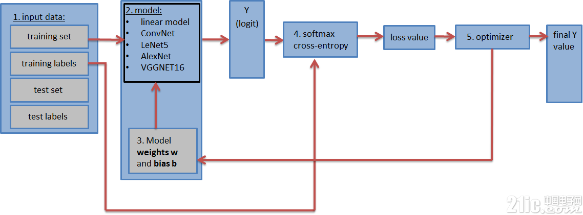
　　包含神经网络的图(如上图所示)应包含以下步骤：

　　1. 输入数据集：训练数据集和标签、测试数据集和标签(以及验证数据集和标签)。 测试和验证数据集可以放在tf.constant()中。而训练数据集被放在tf.placeholder()中，这样它可以在训练期间分批输入(随机梯度下降)。

　　2. 神经网络**模型**及其所有的层。这可以是一个简单的完全连接的神经网络，仅由一层组成，或者由5、9、16层组成的更复杂的神经网络。

　　3. 权重矩阵和**偏差矢量**以适当的形状进行定义和初始化。(每层一个权重矩阵和偏差矢量)

　　4. 损失值：模型可以输出分对数矢量(估计的训练标签)，并通过将分对数与实际标签进行比较，计算出损失值(具有交叉熵函数的softmax)。损失值表示估计训练标签与实际训练标签的接近程度，并用于更新权重值。

　　5. 优化器：它用于将计算得到的损失值来更新反向传播算法中的权重和偏差。

　　2.2 数据加载

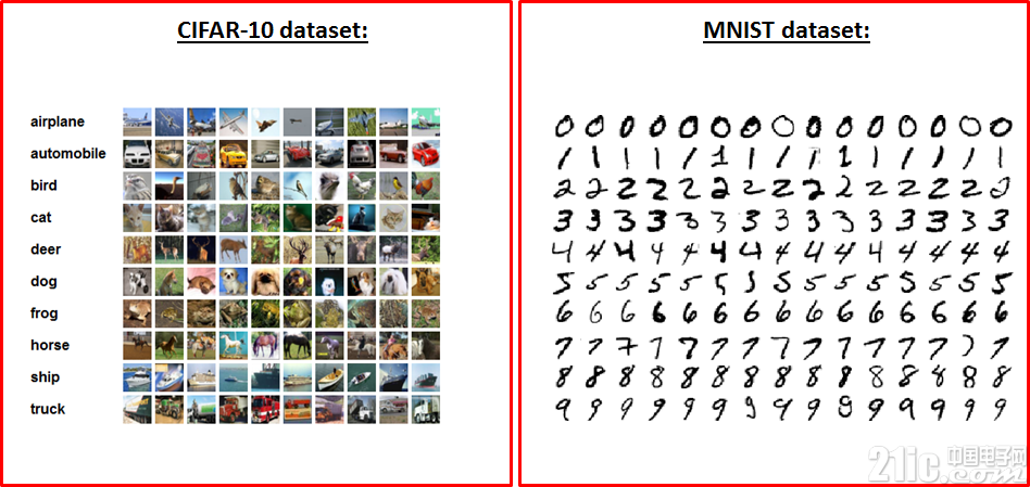
　　下面我们来加载用于训练和测试神经网络的数据集。为此，我们要下载MNIST和CIFAR-10数据集。 MNIST数据集包含了6万个手写数字图像，其中每个图像大小为28 x 28 x 1(灰度)。 CIFAR-10数据集也包含了6万个图像(3个通道)，大小为32 x 32 x 3，包含10个不同的物体(飞机、汽车、鸟、猫、鹿、狗、青蛙、马、船、卡车)。 由于两个数据集中都有10个不同的对象，所以这两个数据集都包含10个标签。

　　首先，我们来定义一些方便载入数据和格式化数据的方法。

　　def randomize(dataset, labels):

　　permutation = np.random.permutation(labels.shape[0])

　　shuffled_dataset = dataset[permutation, :, :]

　　shuffled_labels = labels[permutation]

　　return shuffled_dataset, shuffled_labels

　　def one_hot_encode(np_array):

　　return (np.arange(10) == np_array[:,None]).astype(np.float32)

　　def reformat_data(dataset, labels, image_width, image_height, image_depth):

　　np_dataset_ = np.array([np.array(image_data).reshape(image_width, image_height, image_depth) for image_data in dataset])

　　np_labels_ = one_hot_encode(np.array(labels, dtype=np.float32))

　　np_dataset, np_labels = randomize(np_dataset_, np_labels_)

　　return np_dataset, np_labels

　　def flatten_tf_array(array):

　　shape = array.get_shape().as_list()

　　return tf.reshape(array, [shape[0], shape[1] shape[2] shape[3]])

　　def accuracy(predictions, labels):

　　return (100.0 * np.sum(np.argmax(predictions, 1) == np.argmax(labels, 1)) / predictions.shape[0])

　　这些方法可用于对标签进行独热码编码、将数据加载到随机数组中、扁平化矩阵(因为完全连接的网络需要一个扁平矩阵作为输入)：

　　在我们定义了这些必要的函数之后，我们就可以这样加载MNIST和CIFAR-10数据集了：

　　mnist_folder = './data/mnist/'

　　mnist_image_width = 28

　　mnist_image_height = 28

　　mnist_image_depth = 1

　　mnist_num_labels = 10

　　mndata = MNIST(mnist_folder)

　　mnist_train_dataset_, mnist_train_labels_ = mndata.load_training()

　　mnist_test_dataset_, mnist_test_labels_ = mndata.load_testing()

　　mnist_train_dataset, mnist_train_labels = reformat_data(mnist_train_dataset_, mnist_train_labels_, mnist_image_size, mnist_image_size, mnist_image_depth)

　　mnist_test_dataset, mnist_test_labels = reformat_data(mnist_test_dataset_, mnist_test_labels_, mnist_image_size, mnist_image_size, mnist_image_depth)

　　print("There are {} images, each of size {}".format(len(mnist_train_dataset), len(mnist_train_dataset[0])))

　　print("Meaning each image has the size of 28281 = {}".format(mnist_image_sizemnist_image_size1))

　　print("The training set contains the following {} labels: {}".format(len(np.unique(mnist_train_labels_)), np.unique(mnist_train_labels_)))

　　print('Training set shape', mnist_train_dataset.shape, mnist_train_labels.shape)

　　print('Test set shape', mnist_test_dataset.shape, mnist_test_labels.shape)

　　train_dataset_mnist, train_labels_mnist = mnist_train_dataset, mnist_train_labels

　　test_dataset_mnist, test_labels_mnist = mnist_test_dataset, mnist_test_labels

　　######################################################################################

　　cifar10_folder = './data/cifar10/'

　　train_datasets = ['data_batch_1', 'data_batch_2', 'data_batch_3', 'data_batch_4', 'data_batch_5', ]

　　test_dataset = ['test_batch']

　　c10_image_height = 32

　　c10_image_width = 32

　　c10_image_depth = 3

　　c10_num_labels = 10

　　with open(cifar10_folder + test_dataset[0], 'rb') as f0:

　　c10_test_dict = pickle.load(f0, encoding='bytes')

　　c10_test_dataset, c10_test_labels = c10_test_dict[b'data'], c10_test_dict[b'labels']

　　test_dataset_cifar10, test_labels_cifar10 = reformat_data(c10_test_dataset, c10_test_labels, c10_image_size, c10_image_size, c10_image_depth)

　　c10_train_dataset, c10_train_labels = [], []

　　for train_dataset in train_datasets:

　　with open(cifar10_folder + train_dataset, 'rb') as f0:

　　c10_train_dict = pickle.load(f0, encoding='bytes')

　　c10_train_dataset_, c10_train_labels_ = c10_train_dict[b'data'], c10_train_dict[b'labels']

　　c10_train_dataset.append(c10_train_dataset_)

　　c10_train_labels += c10_train_labels_

　　c10_train_dataset = np.concatenate(c10_train_dataset, axis=0)

　　train_dataset_cifar10, train_labels_cifar10 = reformat_data(c10_train_dataset, c10_train_labels, c10_image_size, c10_image_size, c10_image_depth)

　　del c10_train_dataset

　　del c10_train_labels

　　print("The training set contains the following labels: {}".format(np.unique(c10_train_dict[b'labels'])))

　　print('Training set shape', train_dataset_cifar10.shape, train_labels_cifar10.shape)

　　print('Test set shape', test_dataset_cifar10.shape, test_labels_cifar10.shape)

　　你可以从Yann LeCun的网站下载MNIST数据集。下载并解压缩之后，可以使用python-mnist 工具来加载数据。 CIFAR-10数据集可以从这里下载。