一步一步学用Tensorflow构建卷积神经网络

　　2.6 影响层输出大小的参数

　　一般来说，神经网络的层数越多越好。我们可以添加更多的层、修改激活函数和池层，修改学习速率，以看看每个步骤是如何影响性能的。由于i层的输入是i-1层的输出，我们需要知道不同的参数是如何影响i-1层的输出大小的。

　　要了解这一点，可以看看conv2d()函数。

　　它有四个参数：

　　输入图像，维度为[batch size, image_width, image_height, image_depth]的4D张量

　　权重矩阵，维度为[filter_size, filter_size, image_depth, filter_depth]的4D张量

　　每个维度的步幅数。

　　填充(='SAME'/'VALID')

　　这四个参数决定了输出图像的大小。

　　前两个参数分别是包含一批输入图像的4D张量和包含卷积滤波器权重的4D张量。

　　第三个参数是卷积的步幅，即卷积滤波器在四维的每一个维度中应该跳过多少个位置。这四个维度中的第一个维度表示图像批次中的图像编号，由于我们不想跳过任何图像，因此始终为1。最后一个维度表示图像深度(不是色彩的通道数;灰度为1，RGB为3)，由于我们不想跳过任何颜色通道，所以这个也总是为1。第二和第三维度表示X和Y方向上的步幅(图像宽度和高度)。如果要应用步幅，则这些是过滤器应跳过的位置的维度。因此，对于步幅为1，我们必须将步幅参数设置为[1, 1, 1, 1]，如果我们希望步幅为2，则将其设置为[1，2，2，1]。以此类推。

　　最后一个参数表示Tensorflow是否应该对图像用零进行填充，以确保对于步幅为1的输出尺寸不会改变。如果 padding = 'SAME'，则图像用零填充(并且输出大小不会改变)，如果 padding = 'VALID'，则不填充。

　　下面我们可以看到通过图像(大小为28 x 28)扫描的卷积滤波器(滤波器大小为5 x 5)的两个示例。

　　在左侧，填充参数设置为“SAME”，图像用零填充，最后4行/列包含在输出图像中。

　　在右侧，填充参数设置为“VALID”，图像不用零填充，最后4行/列不包括在输出图像中。

　　我们可以看到，如果没有用零填充，则不包括最后四个单元格，因为卷积滤波器已经到达(非零填充)图像的末尾。这意味着，对于28 x 28的输入大小，输出大小变为24 x 24 。如果 padding = 'SAME'，则输出大小为28 x 28。

　　如果在扫描图像时记下过滤器在图像上的位置(为简单起见，只有X方向)，那么这一点就变得更加清晰了。如果步幅为1，则X位置为0-5、1-6、2-7，等等。如果步幅为2，则X位置为0-5、2-7、4-9，等等。

　　如果图像大小为28 x 28，滤镜大小为5 x 5，并且步长1到4，那么我们可以得到下面这个表：

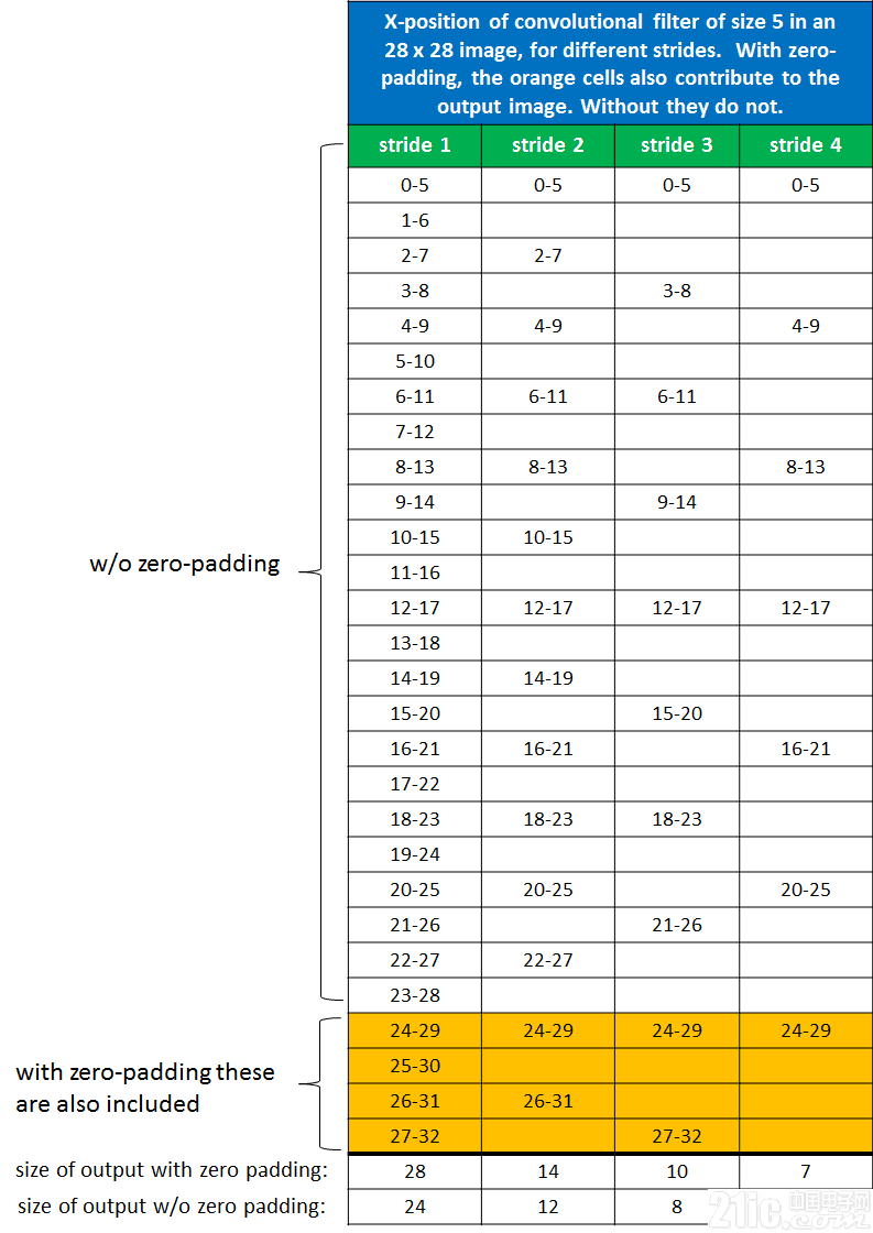
　　可以看到，对于步幅为1，零填充输出图像大小为28 x 28。如果非零填充，则输出图像大小变为24 x 24。对于步幅为2的过滤器，这几个数字分别为 14 x 14 和 12 x 12，对于步幅为3的过滤器，分别为 10 x 10 和 8 x 8。以此类推。

　　对于任意一个步幅S，滤波器尺寸K，图像尺寸W和填充尺寸P，输出尺寸将为

　　如果在Tensorflow中 padding = “SAME”，则分子加起来恒等于1，输出大小仅由步幅S决定。

　　2.7 调整 LeNet5 的架构

　　在原始论文中，LeNet5架构使用了S形激活函数和平均池。 然而，现在，使用relu激活函数则更为常见。 所以，我们来稍稍修改一下LeNet5 CNN，看看是否能够提高准确性。我们将称之为类LeNet5架构：

　　LENET5_LIKE_BATCH_SIZE = 32

　　LENET5_LIKE_FILTER_SIZE = 5

　　LENET5_LIKE_FILTER_DEPTH = 16

　　LENET5_LIKE_NUM_HIDDEN = 120

　　def variables_lenet5_like(filter_size = LENET5_LIKE_FILTER_SIZE,

　　filter_depth = LENET5_LIKE_FILTER_DEPTH,

　　num_hidden = LENET5_LIKE_NUM_HIDDEN,

　　image_width = 28, image_depth = 1, num_labels = 10):

　　w1 = tf.Variable(tf.truncated_normal([filter_size, filter_size, image_depth, filter_depth], stddev=0.1))

　　b1 = tf.Variable(tf.zeros([filter_depth]))

　　w2 = tf.Variable(tf.truncated_normal([filter_size, filter_size, filter_depth, filter_depth], stddev=0.1))

　　b2 = tf.Variable(tf.constant(1.0, shape=[filter_depth]))

　　w3 = tf.Variable(tf.truncated_normal([(image_width // 4)(image_width // 4)filter_depth , num_hidden], stddev=0.1))

　　b3 = tf.Variable(tf.constant(1.0, shape = [num_hidden]))

　　w4 = tf.Variable(tf.truncated_normal([num_hidden, num_hidden], stddev=0.1))

　　b4 = tf.Variable(tf.constant(1.0, shape = [num_hidden]))

　　w5 = tf.Variable(tf.truncated_normal([num_hidden, num_labels], stddev=0.1))

　　b5 = tf.Variable(tf.constant(1.0, shape = [num_labels]))

　　variables = {

　　'w1': w1, 'w2': w2, 'w3': w3, 'w4': w4, 'w5': w5,

　　'b1': b1, 'b2': b2, 'b3': b3, 'b4': b4, 'b5': b5

　　}

　　return variables

　　def model_lenet5_like(data, variables):

　　layer1_conv = tf.nn.conv2d(data, variables['w1'], [1, 1, 1, 1], padding='SAME')

　　layer1_actv = tf.nn.relu(layer1_conv + variables['b1'])

　　layer1_pool = tf.nn.avg_pool(layer1_actv, [1, 2, 2, 1], [1, 2, 2, 1], padding='SAME')

　　layer2_conv = tf.nn.conv2d(layer1_pool, variables['w2'], [1, 1, 1, 1], padding='SAME')

　　layer2_actv = tf.nn.relu(layer2_conv + variables['b2'])

　　layer2_pool = tf.nn.avg_pool(layer2_actv, [1, 2, 2, 1], [1, 2, 2, 1], padding='SAME')

　　flat_layer = flatten_tf_array(layer2_pool)

　　layer3_fccd = tf.matmul(flat_layer, variables['w3']) + variables['b3']

　　layer3_actv = tf.nn.relu(layer3_fccd)

　　#layer3_drop = tf.nn.dropout(layer3_actv, 0.5)

　　layer4_fccd = tf.matmul(layer3_actv, variables['w4']) + variables['b4']

　　layer4_actv = tf.nn.relu(layer4_fccd)

　　#layer4_drop = tf.nn.dropout(layer4_actv, 0.5)

　　logits = tf.matmul(layer4_actv, variables['w5']) + variables['b5']

　　return logits

　　主要区别是我们使用了relu激活函数而不是S形激活函数。

　　除了激活函数，我们还可以改变使用的优化器，看看不同的优化器对精度的影响。

　　2.8 学习速率和优化器的影响

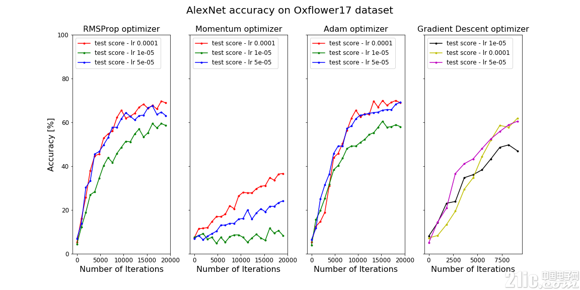
　　让我们来看看这些CNN在MNIST和CIFAR-10数据集上的表现。

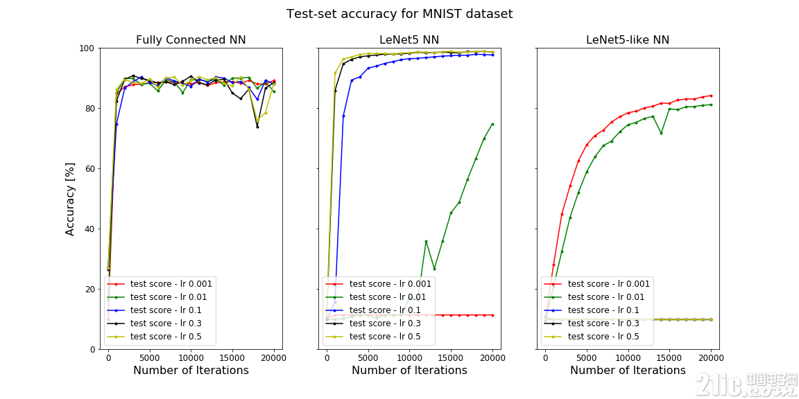
　　在上面的图中，测试集的精度是迭代次数的函数。左侧为一层完全连接的NN，中间为LeNet5 NN，右侧为类LeNet5 NN。

　　可以看到，LeNet5 CNN在MNIST数据集上表现得非常好。这并不是一个大惊喜，因为它专门就是为分类手写数字而设计的。MNIST数据集很小，并没有太大的挑战性，所以即使是一个完全连接的网络也表现的很好。

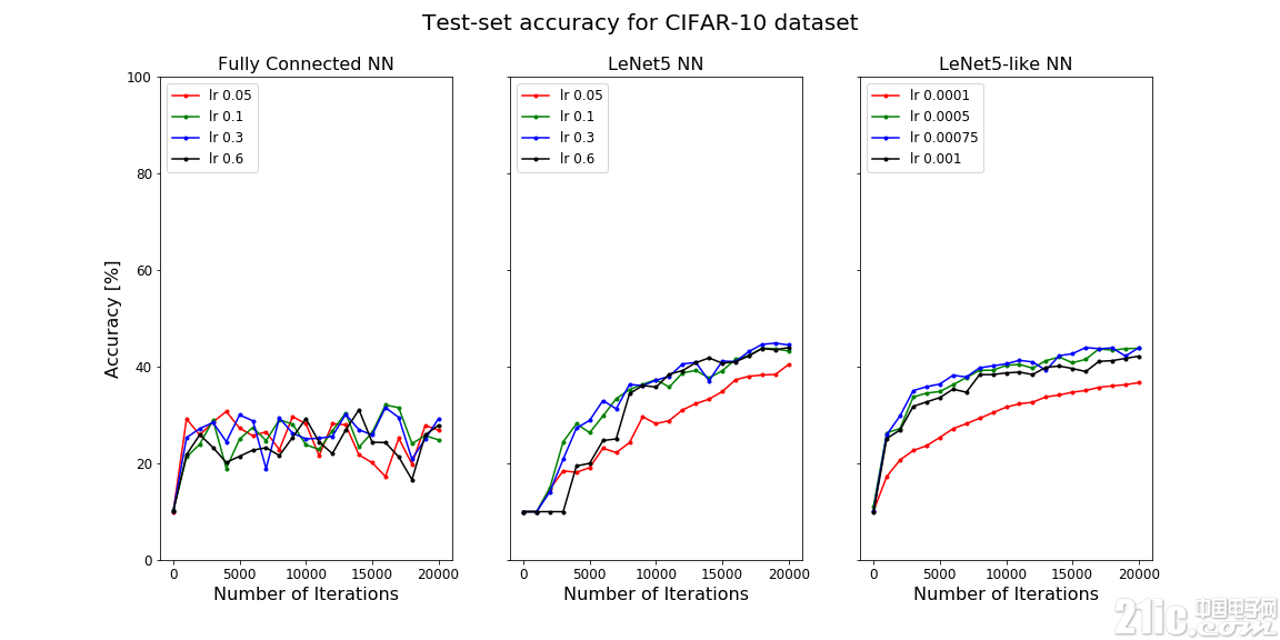
　　然而，在CIFAR-10数据集上，LeNet5 NN的性能显着下降，精度下降到了40%左右。

　　为了提高精度，我们可以通过应用正则化或学习速率衰减来改变优化器，或者微调神经网络。

　　可以看到，AdagradOptimizer、AdamOptimizer和RMSPropOptimizer的性能比GradientDescentOptimizer更好。这些都是自适应优化器，其性能通常比GradientDescentOptimizer更好，但需要更多的计算能力。

　　通过L2正则化或指数速率衰减，我们可能会得到更搞的准确性，但是要获得更好的结果，我们需要进一步研究。

　　3. Tensorflow 中的深度神经网络

　　到目前为止，我们已经看到了LeNet5 CNN架构。 LeNet5包含两个卷积层，紧接着的是完全连接的层，因此可以称为浅层神经网络。那时候(1998年)，GPU还没有被用来进行计算，而且CPU的功能也没有那么强大，所以，在当时，两个卷积层已经算是相当具有创新意义了。

　　后来，很多其他类型的卷积神经网络被设计出来，你可以在这里查看详细信息。

　　比如，由Alex Krizhevsky开发的非常有名的AlexNet 架构(2012年)，7层的ZF Net (2013)，以及16层的 VGGNet (2014)。

　　在2015年，Google发布了一个包含初始模块的22层的CNN(GoogLeNet)，而微软亚洲研究院构建了一个152层的CNN，被称为ResNet。

　　现在，根据我们目前已经学到的知识，我们来看一下如何在Tensorflow中创建AlexNet和VGGNet16架构。

　　3.1 AlexNet

　　虽然LeNet5是第一个ConvNet，但它被认为是一个浅层神经网络。它在由大小为28 x 28的灰度图像组成的MNIST数据集上运行良好，但是当我们尝试分类更大、分辨率更好、类别更多的图像时，性能就会下降。

　　第一个深度CNN于2012年推出，称为AlexNet，其创始人为Alex Krizhevsky、Ilya Sutskever和Geoffrey Hinton。与最近的架构相比，AlexNet可以算是简单的了，但在当时它确实非常成功。它以令人难以置信的15.4%的测试错误率赢得了ImageNet比赛(亚军的误差为26.2%)，并在全球深度学习和人工智能领域掀起了一场革命。

　　它包括5个卷积层、3个最大池化层、3个完全连接层和2个丢弃层。整体架构如下所示：

　　第0层：大小为224 x 224 x 3的输入图像

　　第1层：具有96个滤波器(filter_depth_1 = 96)的卷积层，大小为11×11(filter_size_1 = 11)，步长为4。它包含ReLU激活函数。 紧接着的是最大池化层和本地响应归一化层。

　　第2层：具有大小为5 x 5(filter_size_2 = 5)的256个滤波器(filter_depth_2 = 256)且步幅为1的卷积层。它包含ReLU激活函数。 紧接着的还是最大池化层和本地响应归一化层。

　　第3层：具有384个滤波器的卷积层(filter_depth_3 = 384)，尺寸为3×3(filter_size_3 = 3)，步幅为1。它包含ReLU激活函数

　　第4层：与第3层相同。

　　第5层：具有大小为3×3(filter_size_4 = 3)的256个滤波器(filter_depth_4 = 256)且步幅为1的卷积层。它包含ReLU激活函数

　　第6-8层：这些卷积层之后是完全连接层，每个层具有4096个神经元。在原始论文中，他们对1000个类别的数据集进行分类，但是我们将使用具有17个不同类别(的花卉)的oxford17数据集。

　　请注意，由于这些数据集中的图像太小，因此无法在MNIST或CIFAR-10数据集上使用此CNN(或其他的深度CNN)。正如我们以前看到的，一个池化层(或一个步幅为2的卷积层)将图像大小减小了2倍。 AlexNet具有3个最大池化层和一个步长为4的卷积层。这意味着原始图像尺寸会缩小2^5。 MNIST数据集中的图像将简单地缩小到尺寸小于0。

　　因此，我们需要加载具有较大图像的数据集，最好是224 x 224 x 3(如原始文件所示)。 17个类别的花卉数据集，又名oxflower17数据集是最理想的，因为它包含了这个大小的图像：

　　ox17_image_width = 224

　　ox17_image_height = 224

　　ox17_image_depth = 3

　　ox17_num_labels = 17

　　import tflearn.datasets.oxflower17 as oxflower17

　　train_dataset_, train_labels_ = oxflower17.load_data(one_hot=True)

　　train_dataset_ox17, train_labels_ox17 = train_dataset_[:1000,:,:,:], train_labels_[:1000,:]

　　test_dataset_ox17, test_labels_ox17 = train_dataset_[1000:,:,:,:], train_labels_[1000:,:]

　　print('Training set', train_dataset_ox17.shape, train_labels_ox17.shape)

　　print('Test set', test_dataset_ox17.shape, test_labels_ox17.shape)

　　让我们试着在AlexNet中创建权重矩阵和不同的层。正如我们之前看到的，我们需要跟层数一样多的权重矩阵和偏差矢量，并且每个权重矩阵的大小应该与其所属层的过滤器的大小相对应。

　　ALEX_PATCH_DEPTH_1, ALEX_PATCH_DEPTH_2, ALEX_PATCH_DEPTH_3, ALEX_PATCH_DEPTH_4 = 96, 256, 384, 256

　　ALEX_PATCH_SIZE_1, ALEX_PATCH_SIZE_2, ALEX_PATCH_SIZE_3, ALEX_PATCH_SIZE_4 = 11, 5, 3, 3

　　ALEX_NUM_HIDDEN_1, ALEX_NUM_HIDDEN_2 = 4096, 4096

　　def variables_alexnet(patch_size1 = ALEX_PATCH_SIZE_1, patch_size2 = ALEX_PATCH_SIZE_2,

　　patch_size3 = ALEX_PATCH_SIZE_3, patch_size4 = ALEX_PATCH_SIZE_4,

　　patch_depth1 = ALEX_PATCH_DEPTH_1, patch_depth2 = ALEX_PATCH_DEPTH_2,

　　patch_depth3 = ALEX_PATCH_DEPTH_3, patch_depth4 = ALEX_PATCH_DEPTH_4,

　　num_hidden1 = ALEX_NUM_HIDDEN_1, num_hidden2 = ALEX_NUM_HIDDEN_2,

　　image_width = 224, image_height = 224, image_depth = 3, num_labels = 17):

　　w1 = tf.Variable(tf.truncated_normal([patch_size1, patch_size1, image_depth, patch_depth1], stddev=0.1))

　　b1 = tf.Variable(tf.zeros([patch_depth1]))

　　w2 = tf.Variable(tf.truncated_normal([patch_size2, patch_size2, patch_depth1, patch_depth2], stddev=0.1))

　　b2 = tf.Variable(tf.constant(1.0, shape=[patch_depth2]))

　　w3 = tf.Variable(tf.truncated_normal([patch_size3, patch_size3, patch_depth2, patch_depth3], stddev=0.1))

　　b3 = tf.Variable(tf.zeros([patch_depth3]))

　　w4 = tf.Variable(tf.truncated_normal([patch_size4, patch_size4, patch_depth3, patch_depth3], stddev=0.1))

　　b4 = tf.Variable(tf.constant(1.0, shape=[patch_depth3]))

　　w5 = tf.Variable(tf.truncated_normal([patch_size4, patch_size4, patch_depth3, patch_depth3], stddev=0.1))

　　b5 = tf.Variable(tf.zeros([patch_depth3]))

　　pool_reductions = 3

　　conv_reductions = 2

　　no_reductions = pool_reductions + conv_reductions

　　w6 = tf.Variable(tf.truncated_normal([(image_width // 2no_reductions)(image_height // 2no_reductions)patch_depth3, num_hidden1], stddev=0.1))

　　b6 = tf.Variable(tf.constant(1.0, shape = [num_hidden1]))

　　w7 = tf.Variable(tf.truncated_normal([num_hidden1, num_hidden2], stddev=0.1))

　　b7 = tf.Variable(tf.constant(1.0, shape = [num_hidden2]))

　　w8 = tf.Variable(tf.truncated_normal([num_hidden2, num_labels], stddev=0.1))

　　b8 = tf.Variable(tf.constant(1.0, shape = [num_labels]))

　　variables = {

　　'w1': w1, 'w2': w2, 'w3': w3, 'w4': w4, 'w5': w5, 'w6': w6, 'w7': w7, 'w8': w8,

　　'b1': b1, 'b2': b2, 'b3': b3, 'b4': b4, 'b5': b5, 'b6': b6, 'b7': b7, 'b8': b8

　　}

　　return variables

　　def model_alexnet(data, variables):

　　layer1_conv = tf.nn.conv2d(data, variables['w1'], [1, 4, 4, 1], padding='SAME')

　　layer1_relu = tf.nn.relu(layer1_conv + variables['b1'])

　　layer1_pool = tf.nn.max_pool(layer1_relu, [1, 3, 3, 1], [1, 2, 2, 1], padding='SAME')

　　layer1_norm = tf.nn.local_response_normalization(layer1_pool)

　　layer2_conv = tf.nn.conv2d(layer1_norm, variables['w2'], [1, 1, 1, 1], padding='SAME')

　　layer2_relu = tf.nn.relu(layer2_conv + variables['b2'])

　　layer2_pool = tf.nn.max_pool(layer2_relu, [1, 3, 3, 1], [1, 2, 2, 1], padding='SAME')

　　layer2_norm = tf.nn.local_response_normalization(layer2_pool)

　　layer3_conv = tf.nn.conv2d(layer2_norm, variables['w3'], [1, 1, 1, 1], padding='SAME')

　　layer3_relu = tf.nn.relu(layer3_conv + variables['b3'])

　　layer4_conv = tf.nn.conv2d(layer3_relu, variables['w4'], [1, 1, 1, 1], padding='SAME')

　　layer4_relu = tf.nn.relu(layer4_conv + variables['b4'])

　　layer5_conv = tf.nn.conv2d(layer4_relu, variables['w5'], [1, 1, 1, 1], padding='SAME')

　　layer5_relu = tf.nn.relu(layer5_conv + variables['b5'])

　　layer5_pool = tf.nn.max_pool(layer4_relu, [1, 3, 3, 1], [1, 2, 2, 1], padding='SAME')

　　layer5_norm = tf.nn.local_response_normalization(layer5_pool)

　　flat_layer = flatten_tf_array(layer5_norm)

　　layer6_fccd = tf.matmul(flat_layer, variables['w6']) + variables['b6']

　　layer6_tanh = tf.tanh(layer6_fccd)

　　layer6_drop = tf.nn.dropout(layer6_tanh, 0.5)

　　layer7_fccd = tf.matmul(layer6_drop, variables['w7']) + variables['b7']

　　layer7_tanh = tf.tanh(layer7_fccd)

　　layer7_drop = tf.nn.dropout(layer7_tanh, 0.5)

　　logits = tf.matmul(layer7_drop, variables['w8']) + variables['b8']

　　return logits

　　现在我们可以修改CNN模型来使用AlexNet模型的权重和层次来对图像进行分类。

　　3.2 VGG Net-16

　　VGG Net于2014年由牛津大学的Karen Simonyan和Andrew Zisserman创建出来。 它包含了更多的层(16-19层)，但是每一层的设计更为简单;所有卷积层都具有3×3以及步长为3的过滤器，并且所有最大池化层的步长都为2。

　　所以它是一个更深的CNN，但更简单。

　　它存在不同的配置，16层或19层。 这两种不同配置之间的区别是在第2，第3和第4最大池化层之后对3或4个卷积层的使用(见下文)。

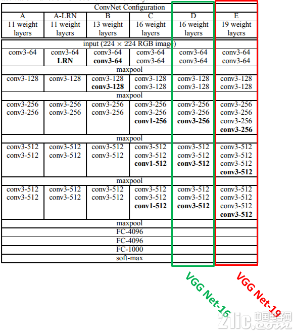
　　配置为16层(配置D)的结果似乎更好，所以我们试着在Tensorflow中创建它。

　　#The VGGNET Neural Network

　　VGG16_PATCH_SIZE_1, VGG16_PATCH_SIZE_2, VGG16_PATCH_SIZE_3, VGG16_PATCH_SIZE_4 = 3, 3, 3, 3

　　VGG16_PATCH_DEPTH_1, VGG16_PATCH_DEPTH_2, VGG16_PATCH_DEPTH_3, VGG16_PATCH_DEPTH_4 = 64, 128, 256, 512

　　VGG16_NUM_HIDDEN_1, VGG16_NUM_HIDDEN_2 = 4096, 1000

　　def variables_vggnet16(patch_size1 = VGG16_PATCH_SIZE_1, patch_size2 = VGG16_PATCH_SIZE_2,

　　patch_size3 = VGG16_PATCH_SIZE_3, patch_size4 = VGG16_PATCH_SIZE_4,

　　patch_depth1 = VGG16_PATCH_DEPTH_1, patch_depth2 = VGG16_PATCH_DEPTH_2,

　　patch_depth3 = VGG16_PATCH_DEPTH_3, patch_depth4 = VGG16_PATCH_DEPTH_4,

　　num_hidden1 = VGG16_NUM_HIDDEN_1, num_hidden2 = VGG16_NUM_HIDDEN_2,

　　image_width = 224, image_height = 224, image_depth = 3, num_labels = 17):

　　w1 = tf.Variable(tf.truncated_normal([patch_size1, patch_size1, image_depth, patch_depth1], stddev=0.1))

　　b1 = tf.Variable(tf.zeros([patch_depth1]))

　　w2 = tf.Variable(tf.truncated_normal([patch_size1, patch_size1, patch_depth1, patch_depth1], stddev=0.1))

　　b2 = tf.Variable(tf.constant(1.0, shape=[patch_depth1]))

　　w3 = tf.Variable(tf.truncated_normal([patch_size2, patch_size2, patch_depth1, patch_depth2], stddev=0.1))

　　b3 = tf.Variable(tf.constant(1.0, shape = [patch_depth2]))

　　w4 = tf.Variable(tf.truncated_normal([patch_size2, patch_size2, patch_depth2, patch_depth2], stddev=0.1))

　　b4 = tf.Variable(tf.constant(1.0, shape = [patch_depth2]))

　　w5 = tf.Variable(tf.truncated_normal([patch_size3, patch_size3, patch_depth2, patch_depth3], stddev=0.1))

　　b5 = tf.Variable(tf.constant(1.0, shape = [patch_depth3]))

　　w6 = tf.Variable(tf.truncated_normal([patch_size3, patch_size3, patch_depth3, patch_depth3], stddev=0.1))

　　b6 = tf.Variable(tf.constant(1.0, shape = [patch_depth3]))

　　w7 = tf.Variable(tf.truncated_normal([patch_size3, patch_size3, patch_depth3, patch_depth3], stddev=0.1))

　　b7 = tf.Variable(tf.constant(1.0, shape=[patch_depth3]))

　　w8 = tf.Variable(tf.truncated_normal([patch_size4, patch_size4, patch_depth3, patch_depth4], stddev=0.1))

　　b8 = tf.Variable(tf.constant(1.0, shape = [patch_depth4]))

　　w9 = tf.Variable(tf.truncated_normal([patch_size4, patch_size4, patch_depth4, patch_depth4], stddev=0.1))

　　b9 = tf.Variable(tf.constant(1.0, shape = [patch_depth4]))

　　w10 = tf.Variable(tf.truncated_normal([patch_size4, patch_size4, patch_depth4, patch_depth4], stddev=0.1))

　　b10 = tf.Variable(tf.constant(1.0, shape = [patch_depth4]))

　　w11 = tf.Variable(tf.truncated_normal([patch_size4, patch_size4, patch_depth4, patch_depth4], stddev=0.1))

　　b11 = tf.Variable(tf.constant(1.0, shape = [patch_depth4]))

　　w12 = tf.Variable(tf.truncated_normal([patch_size4, patch_size4, patch_depth4, patch_depth4], stddev=0.1))

　　b12 = tf.Variable(tf.constant(1.0, shape=[patch_depth4]))

　　w13 = tf.Variable(tf.truncated_normal([patch_size4, patch_size4, patch_depth4, patch_depth4], stddev=0.1))

　　b13 = tf.Variable(tf.constant(1.0, shape = [patch_depth4]))

　　no_pooling_layers = 5

　　w14 = tf.Variable(tf.truncated_normal([(image_width // (2no_pooling_layers))(image_height // (2no_pooling_layers))patch_depth4 , num_hidden1], stddev=0.1))

　　b14 = tf.Variable(tf.constant(1.0, shape = [num_hidden1]))

　　w15 = tf.Variable(tf.truncated_normal([num_hidden1, num_hidden2], stddev=0.1))

　　b15 = tf.Variable(tf.constant(1.0, shape = [num_hidden2]))

　　w16 = tf.Variable(tf.truncated_normal([num_hidden2, num_labels], stddev=0.1))

　　b16 = tf.Variable(tf.constant(1.0, shape = [num_labels]))

　　variables = {

　　'w1': w1, 'w2': w2, 'w3': w3, 'w4': w4, 'w5': w5, 'w6': w6, 'w7': w7, 'w8': w8, 'w9': w9, 'w10': w10,

　　'w11': w11, 'w12': w12, 'w13': w13, 'w14': w14, 'w15': w15, 'w16': w16,

　　'b1': b1, 'b2': b2, 'b3': b3, 'b4': b4, 'b5': b5, 'b6': b6, 'b7': b7, 'b8': b8, 'b9': b9, 'b10': b10,

　　'b11': b11, 'b12': b12, 'b13': b13, 'b14': b14, 'b15': b15, 'b16': b16

　　}

　　return variables

　　def model_vggnet16(data, variables):

　　layer1_conv = tf.nn.conv2d(data, variables['w1'], [1, 1, 1, 1], padding='SAME')

　　layer1_actv = tf.nn.relu(layer1_conv + variables['b1'])

　　layer2_conv = tf.nn.conv2d(layer1_actv, variables['w2'], [1, 1, 1, 1], padding='SAME')

　　layer2_actv = tf.nn.relu(layer2_conv + variables['b2'])

　　layer2_pool = tf.nn.max_pool(layer2_actv, [1, 2, 2, 1], [1, 2, 2, 1], padding='SAME')

　　layer3_conv = tf.nn.conv2d(layer2_pool, variables['w3'], [1, 1, 1, 1], padding='SAME')

　　layer3_actv = tf.nn.relu(layer3_conv + variables['b3'])

　　layer4_conv = tf.nn.conv2d(layer3_actv, variables['w4'], [1, 1, 1, 1], padding='SAME')

　　layer4_actv = tf.nn.relu(layer4_conv + variables['b4'])

　　layer4_pool = tf.nn.max_pool(layer4_pool, [1, 2, 2, 1], [1, 2, 2, 1], padding='SAME')

　　layer5_conv = tf.nn.conv2d(layer4_pool, variables['w5'], [1, 1, 1, 1], padding='SAME')

　　layer5_actv = tf.nn.relu(layer5_conv + variables['b5'])

　　layer6_conv = tf.nn.conv2d(layer5_actv, variables['w6'], [1, 1, 1, 1], padding='SAME')

　　layer6_actv = tf.nn.relu(layer6_conv + variables['b6'])

　　layer7_conv = tf.nn.conv2d(layer6_actv, variables['w7'], [1, 1, 1, 1], padding='SAME')

　　layer7_actv = tf.nn.relu(layer7_conv + variables['b7'])

　　layer7_pool = tf.nn.max_pool(layer7_actv, [1, 2, 2, 1], [1, 2, 2, 1], padding='SAME')

　　layer8_conv = tf.nn.conv2d(layer7_pool, variables['w8'], [1, 1, 1, 1], padding='SAME')

　　layer8_actv = tf.nn.relu(layer8_conv + variables['b8'])

　　layer9_conv = tf.nn.conv2d(layer8_actv, variables['w9'], [1, 1, 1, 1], padding='SAME')

　　layer9_actv = tf.nn.relu(layer9_conv + variables['b9'])

　　layer10_conv = tf.nn.conv2d(layer9_actv, variables['w10'], [1, 1, 1, 1], padding='SAME')

　　layer10_actv = tf.nn.relu(layer10_conv + variables['b10'])

　　layer10_pool = tf.nn.max_pool(layer10_actv, [1, 2, 2, 1], [1, 2, 2, 1], padding='SAME')

　　layer11_conv = tf.nn.conv2d(layer10_pool, variables['w11'], [1, 1, 1, 1], padding='SAME')

　　layer11_actv = tf.nn.relu(layer11_conv + variables['b11'])

　　layer12_conv = tf.nn.conv2d(layer11_actv, variables['w12'], [1, 1, 1, 1], padding='SAME')

　　layer12_actv = tf.nn.relu(layer12_conv + variables['b12'])

　　layer13_conv = tf.nn.conv2d(layer12_actv, variables['w13'], [1, 1, 1, 1], padding='SAME')

　　layer13_actv = tf.nn.relu(layer13_conv + variables['b13'])

　　layer13_pool = tf.nn.max_pool(layer13_actv, [1, 2, 2, 1], [1, 2, 2, 1], padding='SAME')

　　flat_layer = flatten_tf_array(layer13_pool)

　　layer14_fccd = tf.matmul(flat_layer, variables['w14']) + variables['b14']

　　layer14_actv = tf.nn.relu(layer14_fccd)

　　layer14_drop = tf.nn.dropout(layer14_actv, 0.5)

　　layer15_fccd = tf.matmul(layer14_drop, variables['w15']) + variables['b15']

　　layer15_actv = tf.nn.relu(layer15_fccd)

　　layer15_drop = tf.nn.dropout(layer15_actv, 0.5)

　　logits = tf.matmul(layer15_drop, variables['w16']) + variables['b16']

　　return logits

　　3.3 AlexNet 性能

　　作为比较，看一下对包含了较大图片的oxflower17数据集的LeNet5 CNN性能：

　　4. 结语

　　相关代码可以在我的GitHub库中获得，因此可以随意在自己的数据集上使用它。

　　在深度学习的世界中还有更多的知识可以去探索：循环神经网络、基于区域的CNN、GAN、加强学习等等。在未来的博客文章中，我将构建这些类型的神经网络，并基于我们已经学到的知识构建更有意思的应用程序。